By Dr. Dario Cabib, CI Systems (Israel) Ltd.
June 2018
Contents
Scope
Background
Additional relations and definitions
The Model
Contrast estimation assuming RB(λ) is a Planck function at temperature TB
Single pixel methane detection
Measurement of integrated path concentration, probability of detection and false alarm rate
Conclusions
Appendix 1
Appendix 2
Scope
This document provides theoretical analysis for Optical Gas Imaging (OGI) with a passive IR sensor. The goal is to provide the formulation to perform quantitative measurements, and to estimate the sensitivity of the measurement based on the noise performance of the sensor itself.
Background
In many industrial situations there is the need for early detection of the presence of certain hazerdous gases, due to the fact that above certain threshold concentrations they become toxic or flammable (such as methane and other hydrocarbons).
The present model relates the spectral radiance contrast before and after the appearance of methane in a pixel (or, in certain situations between a pixel inside and a pixel outside the cloud) as function of wavelength, methane absorption properties and atmospheric conditions.
Methane is used here as an example, other hydrocarbons or other gases can be treated in a similar way using the same general model. The most important result of this work is that a Long Wave IR (LWIR) camera system, based on a modern uncooled detector array, is sensitive enough to detect and measure methane of such concentration and cloud size which is lower than the Lower Explosive Limit (LEL), and as a result is capable of warning when the threshold is exceeded, indicating a potential dangerous condition.
The advantage of a wavelength dependent model is it can be used to select the most appropriate wavelength region of sensitivity and multispectral capability for the specific gas and meteorological conditions for which the system is designed. A mathematical model fulfills additional functions:
- It provides the algorithm for the estimation of the methane cloud path integrated concentration in the given atmospheric conditions from the radiation measurement data.
- Given a particular measuring equipment with known noise performance it allows the estimation of the detection threshold, cloud concentration*path sensitivity and statistical parameters such as probability of detection and false alarm rate.
- Conversely, given specific requirements of detection threshold and concentration*path sensitivity, it may serve as the basis for a system design with these particular capabilities.
This model is based on the following assumptions:
1a. The background behind any pixel in the cloud is a radiator of spectral radiance RB(λ), where λ is the wavelength.
1b. The methane cloud is a region of space of uniform gas concentration at uniform temperature TC. TC is equal to the air temperature in the location of the cloud.
1c. Any pixel in the cloud is a radiator which partly transmits the background and partly self-emits its own radiation.
1d. The radiance transmitted by the cloud at each wavelength follows Lambert-Beer law and the spectral transmittance is designated τ(λ).
1e. The radiance self-emitted by the cloud at each wavelength is the product of its spectral emissivity ε(λ) by the Planck function at temperature TC, and ε(λ) =1- τ(λ). The latter relation assumes that the cloud does not reflect or scatter any radiation, it transmits some and absorbs some of the incident radiation.
1f. The total radiance reaching the measuring instrument from a pixel is affected by the spectral atmospheric transmittance at the distance of the observed object and it includes a contribution of the self-emission of the air between the observed object and the measuring instrument.
Additional relations and definitions
Blackbody Planck function at temperature T and wavelength λ:P(T,λ),
Radiance of background of cloud: RB(λ),
Wavenumber of radiation: σ=1/ λ,
Volumetric density of methane cloud or number of methane moles: ρ,
Path length of radiation through cloud: ℓ
Distance between cloud and infrared camera: L,
Spectral atmospheric transmittance at distance L: τA (λ,L) at the appropriate atmospheric conditions.
The methane spectral data is taken from the NIST website.
the measurement conditions.
Using these measurement conditions the spectral transmittance and spectral selfemittance (or self- emission) at any cloud concentration and pathlength can be calculated.
Defining now:
Methane mole during measurement: (1)
150mmHg
Ρ0 = ⏤⏤⏤⏤⏤ mole = 0.197 mole
760mmHg
Path length during measurement: ℓ0 =5cm (2)
ρ= volumetri c density of gas cloud = no. of moles , and
measured transmittance spectrum: τ0(σ) (3)
We can write the transmittance spectrum through the gas cloud (using Lambert-Beer’s law):
ρℓ
⏤⏤ (4)
τρ,ℓ(σ) = τ0(σ) ρ0ℓ0
The Model
The cloud measurement configuration with the IR camera is as in the following diagram:
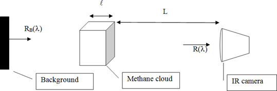
Figure 1. Schematics of radiometric measurement of a cloud against a background.
Designate the radiance originating from a pixel in the cloud and reaching the IR camera plane as R(λ):

Designate the radiance originating from a pixel in the background and reaching the IR camera plane in the absence of cloud as Rb'(λ):
 (6)
(6)
This is obtained neglecting the distance between the background and the cloud, so that τA is the same in both cases or assuming that RB(l) is the background radiance transferred to the cloud plane. Clearly, at wavelengths at which τρλ=1
 (7)
(7)
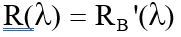
This means, as it should be, that at wavelengths at which the cloud is transparent the radiance from a pixel in the cloud is the same as the radiance from a pixel in the background.
Equation (5) can be simplified to:

The spatial contrast between a pixel in the background outside the cloud and a pixel in the cloud is therefore obtained by subtracting (8) from (6):
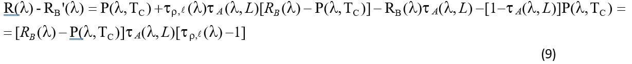
The time contrast of the spectral radiance of a pixel after and before the cloud is present, designated as Δ,R(λ), can be expressed as the difference between the expression of equation (8) with general τρ,ℓ (λ) and the same expression with τρ,ℓ (λ) =1 at every wavelength:

(10) is formally the same as (9). The difference between (9) and (10) is that in (9) RB is the background
assumed to be the same in two different pixels, one in the cloud and one outside.
In (10) RB is the background of the same pixel assumed to be the same before and after the cloud is present.
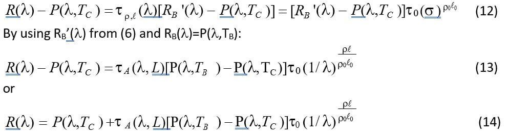
Now we note, from (6) and (8) that:

The left hand side of (11) is known because R(λ), RB’(λ) and TC are measured. Once τρ,ℓ (λ) is known it can be used in equation (4) to find the product Ρℓ by inversion.
It is noteworthy that in this procedure for finding Ρℓ τA(λ,L) does not have to be known, but one has to be careful that (λ) should be such that RB’(λ) and P(λ,TC) are different, otherwise the denominator of (11) is zero.
In general this is true for any wavelength if the background is a blackbody at a temperature different than the cloud/air temperature. This is not a very restrictive condition, since it is known that this type of gas imaging is not useful if the background and gas temperature are the same.
Alternatively, if one cannot rely on background spatial uniformity or background measurement before the cloud appears, then equation (8) must be used pixel by pixel: in this case τρ,ℓ , and as a consequence methane concentration*path length, can be estimated only if we can have a reasonable assumption for RB(λ) and for τA(λ,L).
Contrast estimation assuming RB(λ)
is a Planck function at temperature TB
We rewrite equation (11) as:
Now we will assume a fixed value of TC, a fixed value of Ρℓ , specific atmospheric conditions and a fixed value of L to yield an atmospheric transmittance spectrum τA (λ,L) , and we can plot the right hand of (14) for various values of ΔT=TB-TC. For each of these curves we can also plot the closest Planck function curve P(λ,T) for comparison with R(λ). In Figures 2 and 3, R(λ), P(λ,TB) and P(λ,TC) are plotted as
functions of λ, for Ρℓ =2%.meter as an example TB=30C, TC=20C, and τA(λ,L)=1.
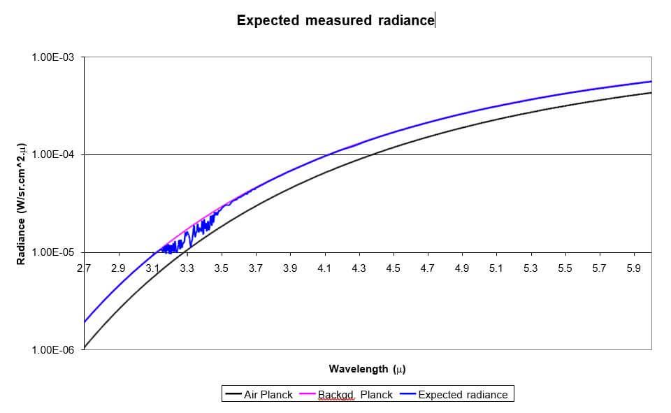
Figure 2. Expected measured Mid Wave IR spectral radiance R(λ) of a methane cloud reaching the IR camera of Figure 1. Background temperature is 30C, air temperature is 20C, methane path integrated concentration is 2%.meter. Atmospheric transmittance is assumed to be 100%.
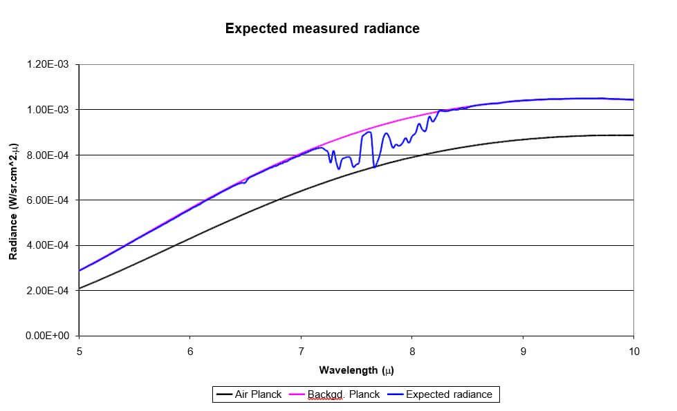
Figure 3. Expected measured Long Wave IR spectral radiance R(λ) of a methane cloud reaching the IR camera of Figure 1. Background temperature is 30C, air temperature is 20C, methane path integrated concentration is 2%.meter. Atmospheric transmittance is assumed to be 1.
As can be seen from Figures 2 and 3 the methane information is in the ranges of 3.1 to 3.6 microns in the Mid Wave and 7.1 to 8.3 microns in the Long Wave IR. Figure 4 shows the transmittance of methane gas in the IR range at the reference path integrated concentration given in NIST website and at 2%.meter, as examples.
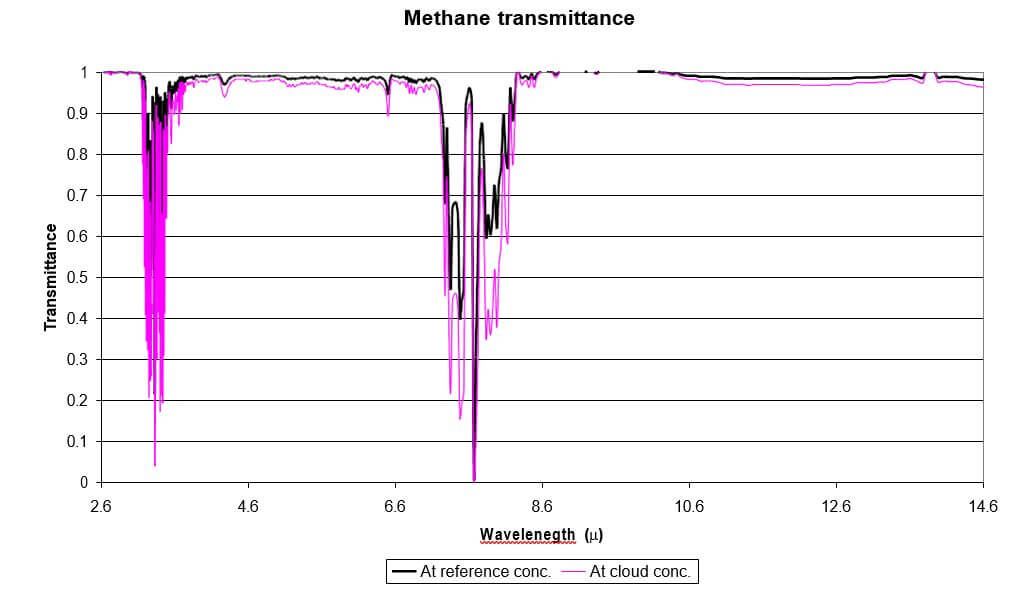
Figure 4. Transmittance spectrum of methane in the measurement of reference conditions given in NIST website (150 mm Hg at 600 mm Hg pressure and 5 cm.) and in the current example of 2%.meter at atmospheric pressure (760 mm Hg), for comparison.
Similar graphs to Figures 2 and 3 may be easily plotted for different background and cloud temperatures. It is to be noted that at wavelengths at which methane is transparent the cloud radiance coincides with the background Planck function. At wavelengths at which methane gas is partially absorbing the cloud radiance is limited from above by the background Planck function and from below by the cloud Planck function. At wavelengths at which methane gas is completely absorbing the cloud radiance coincides with the cloud Planck function. The situation would be reversed if the background temperature were lower than the cloud temperature.
Single pixel methane detection
An infrared camera, combined with a bandpass filter in the wavelength range carrying the methane information, is used to detect the presence of a methane gas region in the air from a distance, pixel by pixel. This is done by constantly monitoring the signal of a pixel through the above filter and by recording the time behavior of such signal.
Equation (14) shows that for constant TB and TC, R(λ) depends only on Ρℓ , the path integrated concentration of the methane gas region.
As a consequence, the integral of R(λ) in the filter wavelength region depends on Ρℓ also.
In this case if Ρℓ starts from zero (absence and slowly increases with time, the signal recorded by the pixel
will start to decrease (if TB>TC) and will start to increase when TB<TC.
At some point, if the methane integrated path concentration of the cloud continues to increase, the signal will differ from the original signal without methane by an amount larger than the noise of the camera.
At this point the camera system will provide an alarm signal, indicating that the methane cloud reached a predetermined threshold level.
For a given methane gas cloud of a given concentration and size the minimum threshold detectable by the camera depends primarily on the sensitivity of the camera system and on the temperature difference TB-TC.
If TB and TC change with time during the measurement, for detection purposes, these two parameters have to be monitored and taken into account in equation (14).
Measurement of integrated path concentration, probability of detection and false alarm rate
The critical parameter for pixel by pixel cloud detection is then the contrast C1,2 obtained by integrating R(λ)- RB’(λ) or ΔtR(λ) of equation (10) between the wavelength limits of the bandpass filter used in the IR camera, λ1 and λ2.

C1,2 is a radiance contrast in units of Watts/(sr.cm2) and it can be translated to an equivalent temperature contrast for small temperature differences, by a first order approximation:
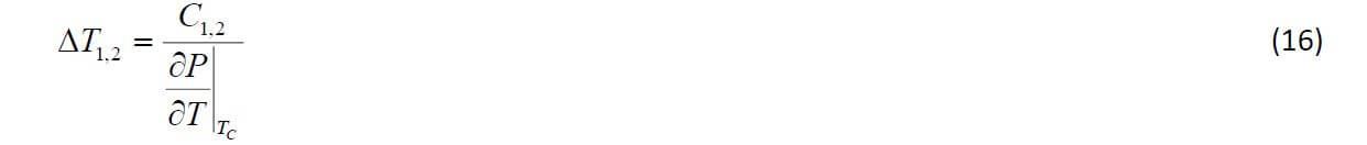
where the partial derivative

is calculated at or in the vicinity of TC.
In order to predict the ability of an infrared camera with filter to detect the contrast of (16), one should compare it with the camera NETD (or Noise Equivalent Temperature Difference). However, this camera NETD is given by the manufacturer for the open camera (without filter), and therefore it must be translated into an equivalent NETD1,2 in the integrated wavelength range of the filter in question (between λ1 and λ2). Since a filtered source produces less radiance at the detector, than when it radiates in an open window, the equivalent NETD in the filter wavelength range is approximately (the responsivity of the IR camera is not entirely “flat” within its spectral range) degraded by a factor equal to the ratio between the radiance in the open camera range and in the filtered range:
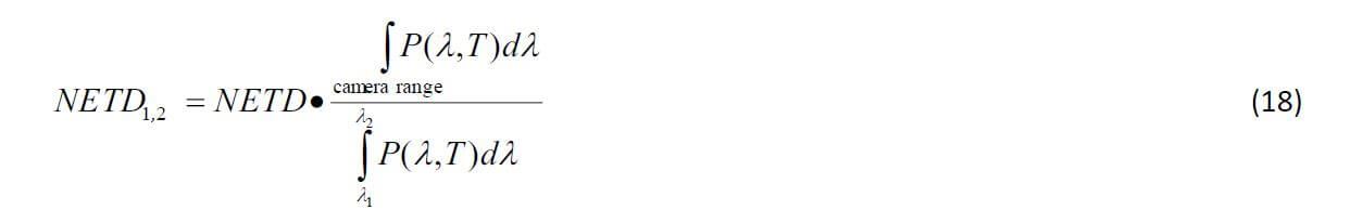
The “camera range” of the integral in the numerator of (18) may be 1 to 5.5 microns of a cooled InSb array camera or the 8 to 14 micron range of an uncooled Long Wave IR camera.
A typical NETD of an uncooled detector array without optics in this range is 50 millikelvin, or 0.05 C.
For methane in the Long Wave range we choose “camera range”= 8 to 14 microns, λ1=7.1 microns, λ2=8.3 microns. The data on the NETD of the camera is given by the manufacturer in the 8 to 14 microns range because this is the standard commercially available range; however, the methane information is in a region partially outside this range. For this reason the useful NETD estimate is done here below in the methane range on the basis of the available data; in addition, the camera manufacturer has that the camera range of sensitivity can be extended to the needed lower range down to 7 microns. (18) then becomes:

An additional factor of 2 due to optical losses by the collection optics of the system and by cloud turbulence may degrade the NETD (as an example):

Values of ρℓ which give a contrast value like in (20) in the 7.1 to 8.3 micron range have been
calculated for different values of TB-TC at TC=20C.
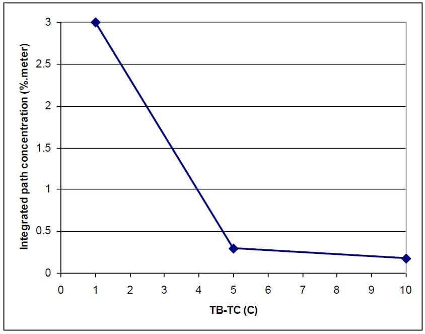
Figure 5. As TB-TC increases the path integrated concentration of a methane cloud that can be detected with a given camera NETD in the 7.1 to 8.3 micron range decreases.
Similar curves can be obtained for a different camera NETD and for different cameras and filter wavelength ranges.
A curve such as in Figure 5 has a tolerance because the camera signals have noise. The contrast values of equations (15) and (16) are obtained by subtracting the signals due to measurements of the radiances in equations (6) and (14). These signals have noise riding on them with certain distributions. We have verified that a typical uncooled LWIR camera pixel produces signals with a noise following a Gaussian distribution law. The law is approximately:

where P(T) is the normalized probability function that a pixel receiving a constant blackbody radiance in laboratory conditions corresponding to a temperature T0 actually gives a signal corresponding to T, and NETD is the Noise Equivalent Temperature Difference of the camera. NETD is equal to σ, the standard deviation of such distribution function.
When comparing two noisy signals through the methane gas absorption line, one before and one after the methane cloud appears, in order to detect the gas we must distinguish between two signals having probability distributions as in Figure 6:
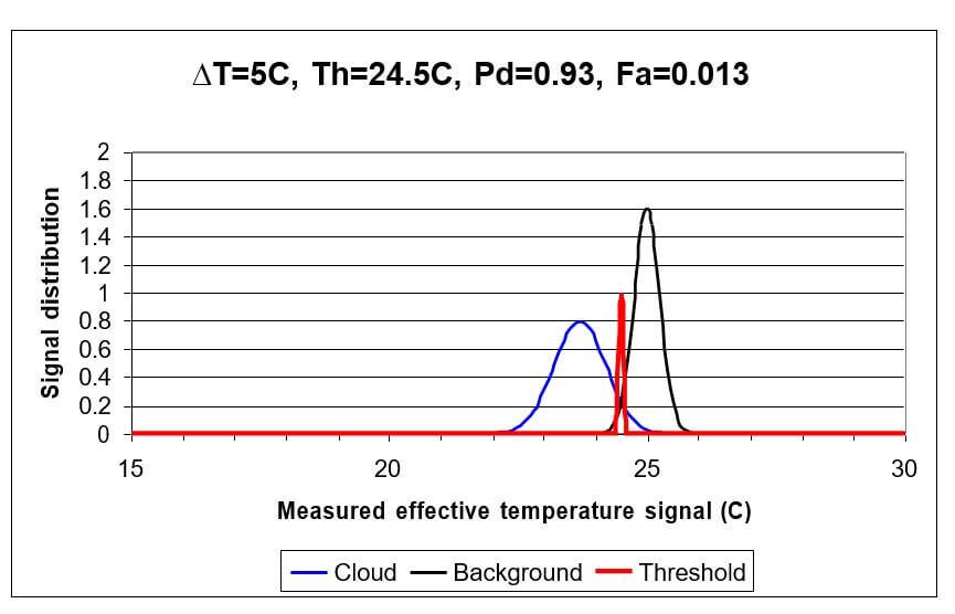
Figure 6. Examples of normalized measured effective temperature signal distributions through the absorption line of a methane cloud (blue) between 7.1 and 8.3 microns and without the cloud in the same spectral range (black): the path integrated concentration of the cloud is 1%.meter. The NETD is assumed to be 0.5C (like in equation (20)) through the cloud and 0.25C without the cloud. The vertical red line is a threshold (Th) defined as the effective temperature reading below which a “methane cloud” is declared and above which a “no cloud” is declared.
In Figure 6 the air temperature is 20C, the background temperature is 25C (ΔT=5C), the effective radiometric cloud temperature is calculated to be 23.7C and the threshold is set at the temperature at which the two curves intersect (24.5C).
From distributions such as the one shown in Figure 6 one can calculate the probability of cloud detection Pd, defined as the integral of the blue curve below the threshold and the false alarm rate Fa as the integral of the black curve below the threshold. In the case of Figure 6 the calculation yields Pd=0.93 and Fa=0.013.
This treatment shows that through the knowledge of the NETD of the measuring system in the different atmospheric situations and the measured effective temperature signals predicted by a radiometric model of radiating objects such as gas clouds measured through infrared absorption lines, the probability of detection and false alarm rates can be predicted.
Conclusions
We have constructed a radiometric model, predicting the signal of a pixel of an IR camera system when imaging a methane cloud through its absorption line as function of path integrated concentration, air and background temperatures. We have also related the noise behavior of a pixel of such camera to the probability of detection and to the false alarm rate of methane in that particular pixel. A possible use of the model is to calculate system performance envelope to help design the system itself. The model provides a basis for an algorithm which translates the signals of a pixel before and after the presence of the cloud into path integrated concentration of the gas. Such model may be enhanced in many different ways by comparing all or some of the signals from the camera pixels among themselves to improve detection probability and false alarm rate, and also by averaging over many measurements over time.
This model has been integrated into our uncooled continuous emissions monitoring system MetCam, along with other propriotery algorithems.
Appendix 1
Correction of the model for finite distance between background and gas cloud
In Figure 1 and equation (5) we assumed a distance L between the cloud and the measuring instrument and we left as undefined the distance between the background and the cloud. The rationale for this is that a uniform background radiance behind the cloud would be transmitted as is up to a plane behind the cloud itself due to the law of conservation of radiance.
However, this approach neglects the atmospheric transmittance through the path length between the background radiator and the cloud. The purpose of this section is to develop the corrected equations in place of equations (5) to (11) in section 3 of this document, pages 3 and 4.
Be L1 the distance between the background.
Be L2 the distance between the cloud and the measuring instrument.
Be L=L1+L2 the total distance between the background radiator and the measuring instrument.
Be the thickness ℓ of the cloud negligible with respect to L1 and L2. Then equation (5) is rewritten
as:
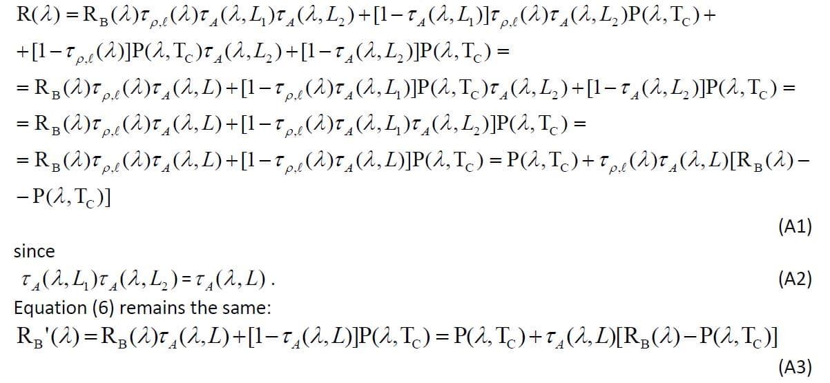
It is to be noted that in the final form of equation (A1) the distance L2 between the cloud and the measuring instrument cancels out and there remains only the distance L to the background. This form is exactly the same as equation (8) of section 3 except that the meaning of L is different than before (it is to the background and not to the cloud).
Obviously then equations (9), (10) and (11) for the contrast and τρ,ℓ (λ) also remain the same with the new meaning of L.
Appendix 2
ESTIMATION OF ERRORS DUE TO AVERAGING IN THE GAS ABSORPTION BAND
Equations (4) and (11) are the basic equations used to derive the cloud’s concentration times path parameter Ρℓ .
These two equations are assumed to express a correct model, but they are valid only for the monochromatic case. In practice the radiometric measurement of R(λ) and RB’(λ) is done in a wavelength band in which the transmittance functions τA(λ,L) and τρ,ℓ (λ) undergo large variations. In addition, the Planck functions and the background radiance in general also undergo variations, although much slower. The purpose of this section is to investigate the methodology for estimating the size of the errors introduced by substituting the wide band data for the monochromatic parameter values. This methodology can then be used to estimate these errors. In a second stage we will try to use these error estimates to improve the accuracy of the measurements.
In practice, the goal is to calculate the difference between the average of τρ,ℓ (λ) calculated as the average of the left hand side and as the ratio of averages in equation (11). In the second stage we have to assess how this difference affects the calculated value of Ρℓ .
From equations (8) and (9) the measured R(λ) and RB’(λ) are integrals over the range of the gas inband filter λ1 and λ2, as follows:
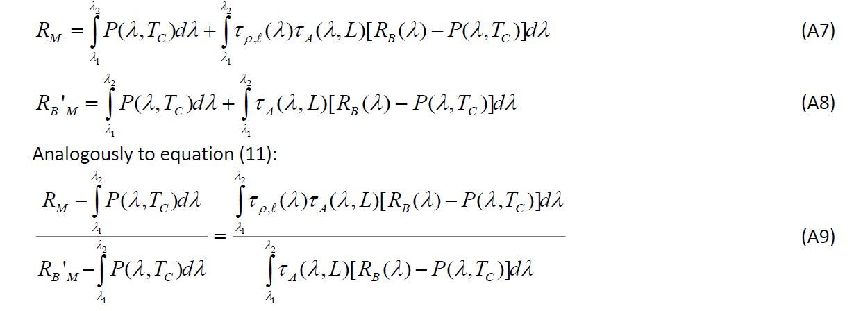
Until here we did not do any approximation: (A9) is still valid according to the original monochromatic model. Now set a value of Ρℓ and calculate the right hand side of (A9) for a range of L’s and % humidities for a given standard atmosphere. (A9) is a weighted average of τρ,ℓ (λ) in the wavelength range of the gas absorption λ1 and λ2, and let us call it << τρ,ℓ (λ) >>.
Now calculate:
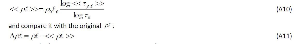
Now plot Δρ,ℓ in the multidimensional space of ρℓ , L, temperature differences between background and air, and atmospheric conditions.